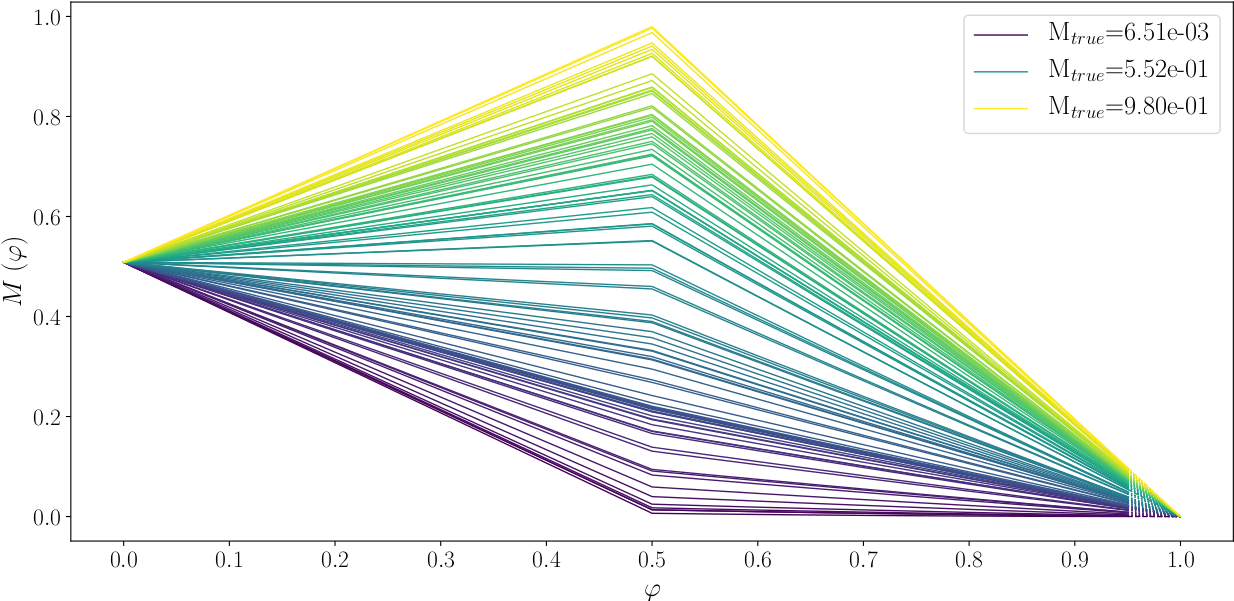
Figure 1: Construction of a series of velocity models M(φ). Each curve shows the evolution of a single velocity value as a function of φ. The model tends to be homogeneous (the same velocity value everywhere) as φ approaches 0 or 1 and the evolutions are linear on the two segments. Values of the true velocity model are found as φ=0.5.
In a previous news about the Full Waveform Inversion (FWI) on surface waves, we showed a preliminary study with real data (“Seignosse” dataset) supplied by RealTimeSeismic. We concluded that more efforts should be made to match the simulation and the real data. We underlined the need of a review on the cost-function due to the characteristics of surface waves. The current cost-function in the code Hawen is constructed in the Frequency-Space (FX) domain while many literatures suggest highly a formulation in the Frequency-Wavenumber (FK) domain for the surface waves. Therefore, we compared the two cost-functions calculated on a series of velocity models M(φ). We have the true model when φ=0.5.
Figure 1 shows the evolution of velocity models as a function of φ. We started from a homogeneous model with an intermediate velocity value and ended at another homogeneous model featuring a low velocity. There were 28 models in all. A forward simulation featuring dozens of frequencies is done for each of them, and the result is compared with the reference simulation performed with the true model. We measured their Euclidean distance in the FX and FK domains respectively. The cost-function curves for each frequency and for all the velocity models are displayed in Figures 2 a and c which show the evolution of the cost-function calculated in the FX domain; b and d show their evolution in the FK domain. Figures 2 c and d highlight the trend of the cost-functions near the true model.
In general, the cost-functions decrease monotonously for high frequencies as the model approaches the true one (at least on the left half of the curves). In case of low frequencies, the trend is more complicated: Figure 2 a indicates that the inversion could stagnate at approximately φ=0.3 if we started the FWI from the left half in the FX domain; Figure 2 b shows that the FWI could go further at low frequencies in the FK domain despite the oscillations after φ=0.4. The right half of the curves indicate unfavourable conditions for the FWI: the curves are nearly flat when φ>0.7, and increasing as φ approaches 0.5 for low frequencies. This infers that we had better avoid starting a FWI from homogeneous models featuring low estimates of velocity. Figure 2 d highlights the major advantage of the cost-function in the FK domain with respect to that in the FX domain shown in Figure 2 c: the “attraction basin” is larger and smoother in the FK domain, which is a favourable condition for the convergence of the FWI result toward the best model.
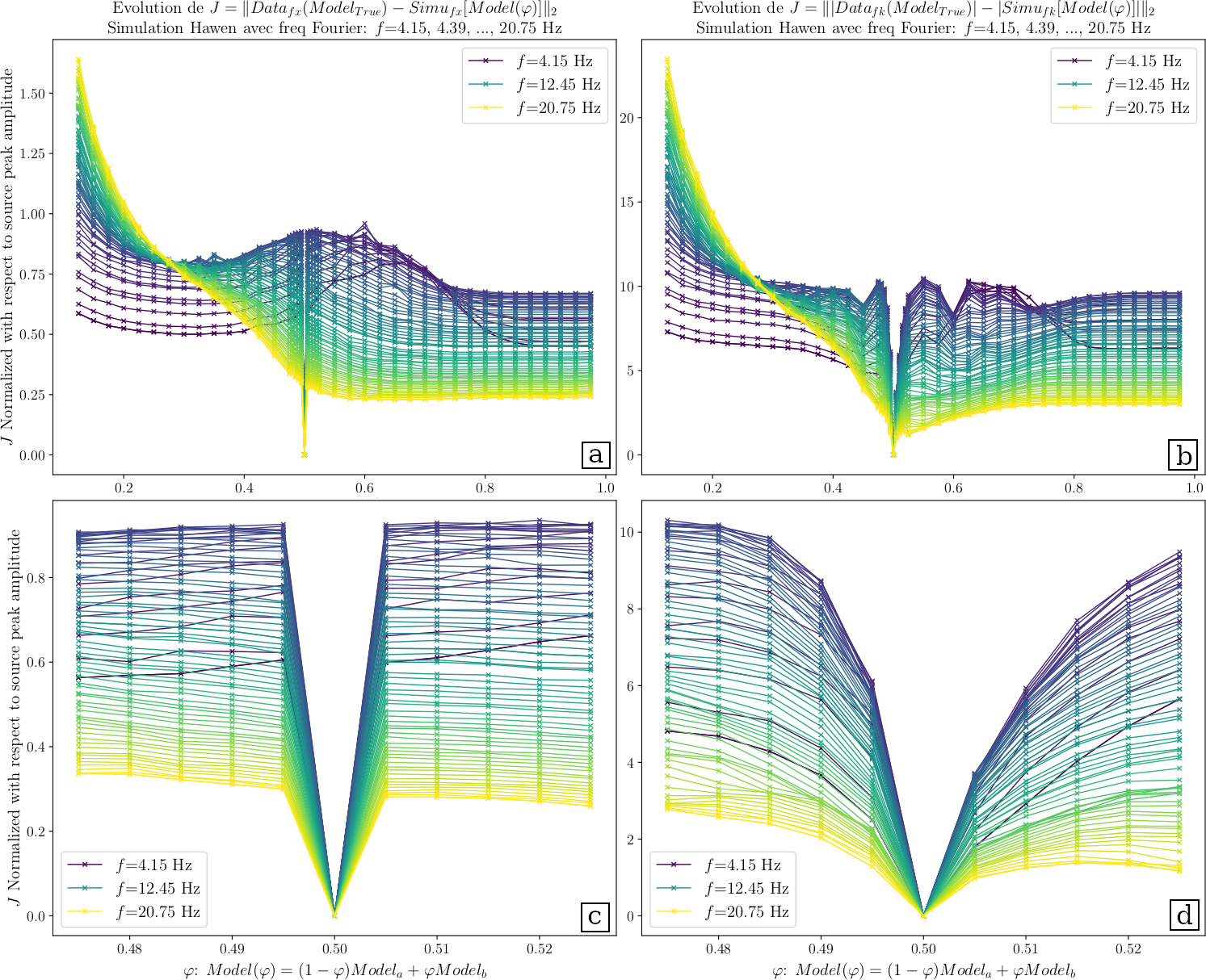
Figure 2: Cost-function curves calculated for a series of velocity models M(φ). Every single curve shows the evolution of a cost-function as a function of φ, namely a given velocity model. Figure 2 a and c correspond to the cost-function constructed in the FX domain while Figure 2 b and d in the FK domain. Figures 2 c and d highlight the central part of Figures 2 a and b, where the models are close to the true model. It is obvious that the “attraction basin”, namely the valley near φ=0.5, is larger and smoother in the FK domain.
In conclusion, the FK domain is potentially the appropriate one in which the FWI featuring strong surface waves may work, as the cost-function shows a larger and smoother “attraction basin”. We constructed a new cost-function in the FK domain and are currently testing it with synthetic data.